A ggplot2 coordinate system that maps a range of IP address space onto a two-dimensional grid using a space-filling curve.
coord_ip() forms the foundation of any ggip plot. It translates all
ip_address and ip_network
vectors to Cartesian coordinates, ready for use by ggplot2 layers (see
Accessing Coordinates). This ensures all layers use a common mapping.
Usage
coord_ip(
  canvas_network = ip_network("0.0.0.0/0"),
  pixel_prefix = 16,
  curve = c("hilbert", "morton"),
  expand = FALSE
)
Arguments
- canvas_network
An
ip_networkscalar that determines the region of IP space visualized by the entire 2D grid. The default shows the entire IPv4 address space.- pixel_prefix
An integer scalar that sets the prefix length of the network represented by a single pixel. The default value is 16. Increasing this effectively improves the resolution of the plot.
- curve
A string to choose the space-filling curve. Choices are
"hilbert"(default) and"morton".- expand
If
TRUE, adds a small expanded margin around the data grid. The default isFALSE.
Accessing Coordinates
coord_ip() stores the result of the mapping in a nested data frame column.
This means each ip_address or
ip_network column in the original data set is
converted to a data frame column. When specifying ggplot2 aesthetics, you'll
need to use $ to access the nested data (see Examples).
Each ip_address column will be replaced with a
data frame containing the following columns:
| Column name | Data type | Description |
ip | ip_address | Original IP data |
x | integer | Pixel x |
y | integer | Pixel y |
Each ip_network column will be replaced with a
data frame containing the following columns:
| Column name | Data type | Description |
ip | ip_network | Original IP data |
xmin | integer | Bounding box xmin |
ymin | integer | Bounding box ymin |
xmax | integer | Bounding box xmax |
ymax | integer | Bounding box ymax |
See also
vignette("visualizing-ip-data") describes the mapping in more detail.
Examples
suppressPackageStartupMessages(library(dplyr))
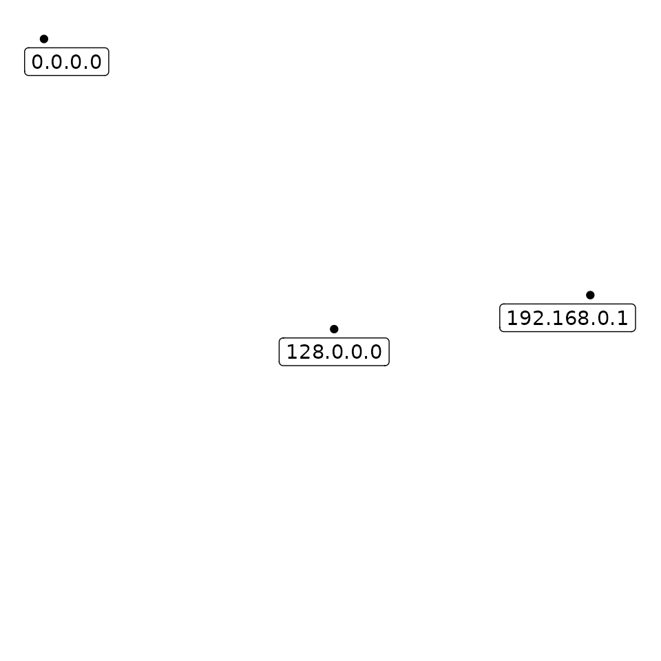
tibble(address = ip_address(c("0.0.0.0", "128.0.0.0", "192.168.0.1"))) %>%
ggplot(aes(x = address$x, y = address$y, label = address$ip)) +
geom_point() +
geom_label(nudge_x = c(10, 0, -10), nudge_y = -10) +
coord_ip(expand = TRUE) +
theme_ip_light()
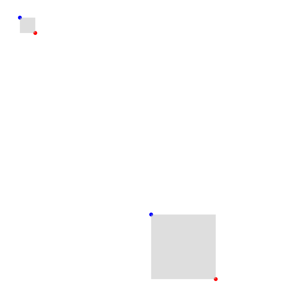
 tibble(network = ip_network(c("0.0.0.0/8", "224.0.0.0/4"))) %>%
mutate(
start = network_address(network),
end = broadcast_address(network)
) %>%
ggplot() +
geom_point(aes(x = start$x, y = start$y), color = "blue") +
geom_point(aes(x = end$x, y = end$y), color = "red") +
geom_rect(
aes(xmin = network$xmin, xmax = network$xmax, ymin = network$ymin, ymax = network$ymax),
alpha = 0.5, fill = "grey"
) +
coord_ip(curve = "morton", expand = TRUE) +
theme_ip_light()
tibble(network = ip_network(c("0.0.0.0/8", "224.0.0.0/4"))) %>%
mutate(
start = network_address(network),
end = broadcast_address(network)
) %>%
ggplot() +
geom_point(aes(x = start$x, y = start$y), color = "blue") +
geom_point(aes(x = end$x, y = end$y), color = "red") +
geom_rect(
aes(xmin = network$xmin, xmax = network$xmax, ymin = network$ymin, ymax = network$ymax),
alpha = 0.5, fill = "grey"
) +
coord_ip(curve = "morton", expand = TRUE) +
theme_ip_light()